The Tsetlin library

Introduction

In this section, we study a simple random walk (or Markov chain), called the Tsetlin library. It will give us the opportunity to see the interplay between combinatorics, linear algebra, representation theory and computer exploration, without requiring heavy theoretical background. I hope this encourages everyone to play around with this or similar systems and investigate their properties! Formal theorems and proofs can be found in the references at the end of this section.

It has been known for several years that the theory of group representations can facilitate the study of systems whose evolution is random (Markov chains), breaking them down into simpler systems. More recently it was realized that generalizing this (namely replacing the invertibility axiom for groups by other axioms) explains the behavior of other particularly simple Markov chains such as the Tsetlin library.

The Tsetlin library

Consider a bookshelf in a library containing \(n\) distinct books. When a person borrows a book and then returns it, it gets placed back on the shelf to the right of all books. This is what we naturally do with our pile of shirts in the closet: after use and cleaning, the shirt is placed on the top of its pile. Hence the most popular books/shirts will more likely appear on the right/top of the shelf/pile.

This type of organization has the advantage of being self-adaptive:

• The books most often used accumulate on the right and thus can easily be found.

• If the use changes over time, the system adapts.

In fact, this type of strategy is used not only in everyday life, but also in computer science. The natural questions that arise are:

• Stationary distribution: To which state(s) does the system converge to? This, among other things, is used to evaluate the average access time to a book.

• The rate of convergence: How fast does the system adapt to a changing environment .

Let us formalize the description. The Tsetlin library is a discrete Markov chain (discrete time, discrete state space) described by:

• The state space \(\Omega_n\) is given by the set of all permutations of the \(n\) books.

• The transition operators are denoted by \(\partial_i \colon \Omega_n \to \Omega_n\). When \(\partial_i\) is applied to a permutation \(\sigma\), the number \(i\) is moved to the end of the permutation.

• We assign parameters \(x_i \ge 0\) for all \(1\le i\le n\) with \(\sum_{i=1}^n x_i = 1\). The parameter \(x_i\) indicates the probability of choosing the operator \(\partial_i\).

Transition graph and matrix

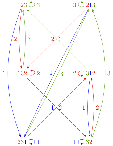
One can depict the action of the operators \(\partial_i\) on the state space \(\Omega_n\) by a digraph. The following picture shows the action of \(\partial_1, \partial_2, \partial_3\) on \(\Omega_3\):

The above picture can be reproduced in Sage as follows:

Sage

sage: P = Poset(([1,2,3],[]))

Python

>>> from sage.all import *
>>> P = Poset(([Integer(1),Integer(2),Integer(3)],[]))

Sage Live

P = Poset(([1,2,3],[]))

This is the antichain poset. Its linear extensions are all permutations of \(\{1,2,3\}\):

Sage

sage: L = P.linear_extensions()
sage: L
The set of all linear extensions of Finite poset containing 3 elements
sage: L.list()
[[3, 2, 1], [3, 1, 2], [1, 3, 2], [1, 2, 3], [2, 1, 3], [2, 3, 1]]

Python

>>> from sage.all import *
>>> L = P.linear_extensions()
>>> L
The set of all linear extensions of Finite poset containing 3 elements
>>> L.list()
[[3, 2, 1], [3, 1, 2], [1, 3, 2], [1, 2, 3], [2, 1, 3], [2, 3, 1]]

Sage Live

L = P.linear_extensions()
L
L.list()

The graph is produced via:

Sage

sage: G = L.markov_chain_digraph(labeling='source'); G
Looped multi-digraph on 6 vertices
sage: view(G)  # not tested

Python

>>> from sage.all import *
>>> G = L.markov_chain_digraph(labeling='source'); G
Looped multi-digraph on 6 vertices
>>> view(G)  # not tested

Sage Live

G = L.markov_chain_digraph(labeling='source'); G
view(G)  # not tested

We can now look at the transition matrix and see whether we notice anything about its eigenvalue and eigenvectors:

Sage

sage: M = L.markov_chain_transition_matrix(labeling='source')
sage: M
[-x0 - x1       x2        0        0       x2        0]
[      x1 -x0 - x2       x1        0        0        0]
[       0        0 -x0 - x1       x2        0       x2]
[      x0        0       x0 -x1 - x2        0        0]
[       0        0        0       x1 -x0 - x2       x1]
[       0       x0        0        0       x0 -x1 - x2]

Python

>>> from sage.all import *
>>> M = L.markov_chain_transition_matrix(labeling='source')
>>> M
[-x0 - x1       x2        0        0       x2        0]
[      x1 -x0 - x2       x1        0        0        0]
[       0        0 -x0 - x1       x2        0       x2]
[      x0        0       x0 -x1 - x2        0        0]
[       0        0        0       x1 -x0 - x2       x1]
[       0       x0        0        0       x0 -x1 - x2]

Sage Live

M = L.markov_chain_transition_matrix(labeling='source')
M

This matrix is normalized so that all columns add to 0. So we need to add \((x_0 + x_1 + x_2)\) times the \(6\times 6\) identity matrix to get the probability matrix:

Sage

sage: x = M.base_ring().gens()
sage: Mt = (x[0]+x[1]+x[2])*matrix.identity(6)+M
sage: Mt
[x2 x2  0  0 x2  0]
[x1 x1 x1  0  0  0]
[ 0  0 x2 x2  0 x2]
[x0  0 x0 x0  0  0]
[ 0  0  0 x1 x1 x1]
[ 0 x0  0  0 x0 x0]

Python

>>> from sage.all import *
>>> x = M.base_ring().gens()
>>> Mt = (x[Integer(0)]+x[Integer(1)]+x[Integer(2)])*matrix.identity(Integer(6))+M
>>> Mt
[x2 x2  0  0 x2  0]
[x1 x1 x1  0  0  0]
[ 0  0 x2 x2  0 x2]
[x0  0 x0 x0  0  0]
[ 0  0  0 x1 x1 x1]
[ 0 x0  0  0 x0 x0]

Sage Live

x = M.base_ring().gens()
Mt = (x[0]+x[1]+x[2])*matrix.identity(6)+M
Mt

Since the \(x_i\) are formal variables, we need to compute the eigenvalues and eigenvectors in the symbolic ring SR:

Sage

sage: Mt.change_ring(SR).eigenvalues()
[x2, x1, x0, x0 + x1 + x2, 0, 0]

Python

>>> from sage.all import *
>>> Mt.change_ring(SR).eigenvalues()
[x2, x1, x0, x0 + x1 + x2, 0, 0]

Sage Live

Mt.change_ring(SR).eigenvalues()

Do you see any pattern? In fact, if you start playing with bigger values of \(n\) (the size of the underlying permutations), you might observe that there is an eigenvalue for every subset \(S\) of \(\{1,2,\ldots,n\}\) and the multiplicity is given by a derangement number \(d_{n-|S|}\). Derangment numbers count permutations without fixed point. For the eigenvectors we obtain:

Sage

sage: Mt.change_ring(SR).eigenvectors_right()
[(x2, [(1, 0, -1, 0, 0, 0)], 1),
 (x1, [(0, 1, 0, 0, -1, 0)], 1),
 (x0, [(0, 0, 0, 1, 0, -1)], 1),
 (x0 + x1 + x2,
  [(1,
    (x0 + x1)/(x0 + x2),
    x0/x1,
    (x0^2 + x0*x1)/(x1^2 + x1*x2),
    (x0^2 + x0*x1)/(x0*x2 + x2^2),
    (x0^2 + x0*x1)/(x1*x2 + x2^2))], 1),
 (0, [(1, 0, -1, 0, -1, 1), (0, 1, -1, 1, -1, 0)], 2)]

Python

>>> from sage.all import *
>>> Mt.change_ring(SR).eigenvectors_right()
[(x2, [(1, 0, -1, 0, 0, 0)], 1),
 (x1, [(0, 1, 0, 0, -1, 0)], 1),
 (x0, [(0, 0, 0, 1, 0, -1)], 1),
 (x0 + x1 + x2,
  [(1,
    (x0 + x1)/(x0 + x2),
    x0/x1,
    (x0^2 + x0*x1)/(x1^2 + x1*x2),
    (x0^2 + x0*x1)/(x0*x2 + x2^2),
    (x0^2 + x0*x1)/(x1*x2 + x2^2))], 1),
 (0, [(1, 0, -1, 0, -1, 1), (0, 1, -1, 1, -1, 0)], 2)]

Sage Live

Mt.change_ring(SR).eigenvectors_right()

The stationary distribution is the eigenvector of eigenvalues \(1=x_0+x_1+x_2\). Do you see a pattern?

Optional exercices: Study of the transition operators and graph

Instead of using the methods that are already in Sage, try to build the state space \(\Omega_n\) and the transition operators \(\partial_i\) yourself as follows.

1. For technical reasons, it is most practical in Sage to label the \(n\) books in the library by \(0,1,\cdots,n-1\), and to represent each state in the Markov chain by a permutation of the set \(\{0,\dots,n-1\}\) as a tuple. Construct the state space \(\Omega_n\) as:

   Sage

   sage: list(map(tuple, Permutations(range(3))))
   [(0, 1, 2), (0, 2, 1), (1, 0, 2), (1, 2, 0), (2, 0, 1), (2, 1, 0)]
   

   Python

   >>> from sage.all import *
   >>> list(map(tuple, Permutations(range(Integer(3)))))
   [(0, 1, 2), (0, 2, 1), (1, 0, 2), (1, 2, 0), (2, 0, 1), (2, 1, 0)]
   

   Sage Live

   list(map(tuple, Permutations(range(3))))

2. Write a function transition_operator(sigma, i) which implements the operator \(\partial_i\) which takes as input a tuple sigma and integer \(i \in \{1,2,\ldots,n\}\) and outputs a new tuple. It might be useful to extract subtuples (sigma[i:j]) and concatenation.

3. Write a function tsetlin_digraph(n) which constructs the (multi digraph) as described as shown above. This can be achieved using DiGraph.

4. Verify for which values of \(n\) the digraph is strongly connected (i.e., you can go from any vertex to any other vertex by going in the direction of the arrow). This indicates whether the Markov chain is irreducible.

Conclusion

The Tsetlin library was studied from the viewpoint of monoids in [Bidigare1997] and [Brown2000]. Precise statements of the eigenvalues and the stationary distribution of the probability matrix as well as proofs of the statements are given in these papers. Generalizations of the Tsetlin library from the antichain to arbitrary posets was given in [AKS2013].

[Bidigare1997]

Thomas Patrick Bidigare. Hyperplane arrangement face algebras and their associated Markov chains. ProQuest LLC, Ann Arbor, MI, 1997. Thesis (Ph.D.) University of Michigan.

[Brown2000]

Kenneth S. Brown. Semigroups, rings, and Markov chains. J. Theoret. Probab., 13(3):871-938, 2000.

[AKS2013]

Arvind Ayyer, Steven Klee, Anne Schilling. Combinatorial Markov chains on linear extensions J. Algebraic Combinatorics, doi:10.1007/s10801-013-0470-9, arXiv 1205.7074.

Make live